1. Introduction¶

In this section we provide an introduction that establishes some initial ideas about how the finite element method works and what it is about.

The finite element method is an approach to solving partial differential equations (PDEs) on complicated domains. It has the flexibility to build discretisations that can increase the order of accuracy, and match the numerical discretisation to the physical problem being modelled. It has an elegant mathematical formulation that lends itself both to mathematical analysis and to flexible code implementation. In this course we blend these two directions together.

1.1. Poisson’s equation in the unit square¶

In this introduction we concentrate on the specific model problem of Poisson’s equation in the unit square.

Definition 1.1 (Poisson’s equation in the unit square)

Let \(\Omega=[0,1]\times[0,1]\). For a given function \(f\), we seek \(u\) such that

(1.1)¶\[-\left(\frac{\partial^2}{\partial x^2}+\frac{\partial^2}{\partial y^2}\right)u:=-\nabla^2 u = f, \quad u(0,y)=u(1,y)=0, \, \frac{\partial u}{\partial y}(x,0)=\frac{\partial u}{\partial y}(x,1)=0.\]

In this problem, the idea is that we are given a specific known function \(f\) (for example, \(f = sin(2\pi x)sin(2 \pi y)\)), and we have to find the corresponding unknown function \(u\) that satisfies the equation (including the boundary conditions). Here we have combined a mixture of Dirichlet boundary conditions specifying the value of the function \(u\), and Neumann boundary conditions specifying the value of the normal derivative \(\partial u/\partial n\). This is because these two types of boundary conditions are treated differently in the finite element method, and we would like to expose both treatments in the same example. The treatment of boundary conditions is one of the strengths of the finite element method.

1.2. Triangulations¶

The description of our finite element method starts by considering a triangulation.

Definition 1.2 (Triangulation)

Let \(\Omega\) be a polygonal subdomain of \(\mathbb{R}^2\). A triangulation \(\mathcal{T}\) of \(\Omega\) is a set of triangles \(\{K_i\}_{i=1}^N\), such that:

\(\mathrm{int}\, K_i \cap \mathrm{int}\, K_j = \emptyset, \quad i\neq j\), where \(\mathrm{int }\) denotes the interior of a set (no overlaps).
\(\cup K_i = \bar{\Omega}\), the closure of \(\Omega\) (triangulation covers \(\Omega\)).
No vertex of any triangle lies in the interior of an edge of another triangle (triangle vertices only meet other triangle vertices).

1.3. Our first finite element space¶

The idea is that we will approximate functions which are polynomial (at some chosen degree) when restricted to each triangle, with some chosen continuity conditions between triangles. We shall call the space of possible functions under these choices a finite element space. In this introduction, we will just consider the following space.

Definition 1.3 (The (P1) finite element space)

Let \(\mathcal{T}\) be a triangulation of \(\Omega\). Then the P1 finite element space is a space \(V_h\) containing all functions \(v\) such that

\(v\in C^0(\Omega)\),
\(v|_{K_i}\) is a linear function for each \(K_i\in \mathcal{T}\).

We also define the following subspace,

(1.2)¶\[\mathring{V}_h = \left\{ v\in V_h: v(0,y)=v(1,y)=0 \right\}.\]

This is the subspace of the P1 finite element space \(V_h\) of functions that satisfy the Dirichlet boundary conditions. We will search only amongst \(\mathring{V}_h\) for our approximate solution to the Poisson equation. This is referred to as strong boundary conditions. Note that we do not consider any subspaces related to the Neumann conditions. These will emerge later.

1.4. Integral formulations and \(L_2\)¶

The finite element method is based upon integral formulations of partial differential equations. Rather than checking if two functions are equal by checking their value at every point, we will just check that they are equal in an integral sense. We do this by introducing the \(L^2\) norm, which is a way of measuring the “magnitude” of a function.

Definition 1.4

For a real-valued function \(f\) on a domain \(\Omega\), with Lebesgue integral

\[\int_\Omega f(x)\,dx,\]

we define the \(L^2\) norm of \(f\),

\[\|f\|_{L^2(\Omega)} = \left(\int_\Omega |f(x)|^2\,dx \right)^{1/2}.\]

This motivates us to say that two functions are equal if the \(L^2\) norm of their difference is zero. It only makes sense to do that if the functions individually have finite \(L^2\) norm, which then also motivates the \(L^2\) function space.

Definition 1.5

We define \(L^2(\Omega)\) as the set of functions

\[L^2(\Omega) = \left\{ f:\|f\|_{L^2(\Omega)}<\infty\right\},\]

and identify two functions \(f\) and \(g\) if \(\|f-g\|_{L^2(\Omega)}=0\), in which case we write \(f\equiv g\) in \(L^2\).

Example 1.6

Consider the two functions \(f\) and \(g\) defined on \(\Omega=[0,1]\times[0,1]\) with

\[\begin{split}f(x,y) = \left\{\begin{array}{cc} 1 & x\geq 0.5, \\ 0 & x < 0.5, \\ \end{array}\right. \, g(x,y) = \left\{\begin{array}{cc} 1 & x> 0.5, \\ 0 & x \leq 0.5. \\ \end{array}\right.\end{split}\]

Since \(f\) and \(g\) only differ on the line \(x=0.5\) which has zero area, then \(\|f-g\|_{L^2(\Omega)}=0\), and so \(f\equiv g\) in \(L^2\).

1.5. Finite element derivative¶

Functions in \(V_h\) do not have derivatives everywhere. This means that we have to work with a more general definition (and later we shall learn when it does and does not work).

Definition 1.7 (Finite element partial derivative)

The finite element partial derivative \(\frac{\partial^{FE}}{\partial x_i}u\) of \(u\) is defined in \(L^2(\Omega)\) such that restricted to \(K_i\), we have

\[\frac{\partial^{FE}u}{\partial x_i}|_{K_i}= \frac{\partial u}{\partial x_i}.\]

Here we see why we needed to introduce \(L^2\): we have a definition that does not have a unique value on the edge between two adjacent triangles. This is verified in the following exercises.

Exercise 1.8

Let \(V_h\) be a P1 finite element space for a triangulation \(\mathcal{T}\) of \(\Omega\). For all \(u\in V_h\), show that the definition above uniquely defines \(\frac{\partial^{FE}u}{\partial x_i}\) in \(L^2(\Omega)\).

Exercise 1.9

Let \(u\in C^1(\Omega)\) (the space of functions with continuous partial derivatives at every point in \(\Omega\)). Show that the finite element partial derivative and the usual derivative are equal in \(L^2(\Omega)\).

In view of this second exercise, in this section we will consider all derivatives to be finite element derivatives. In later sections we shall consider an even more general definition of the derivative which contains both of these definitions.

1.6. Towards the finite element discretisation¶

We will now use the finite element derivative to develop the finite element discretisation. We assume that we have a solution \(u\) to Equation (1.1) that is sufficiently smooth (e.g. \(u\in C^1\) in this case). (Later, we will consider more general types of solutions to this equation, but this assumption just motivates things for the time being.)

We take \(v\in \mathring{V}_h\), multiply by Equation (1.1), and integrate over the domain. Integration by parts in each triangle then gives

\[\sum_{i}\left(\int_{K_i} \nabla v\cdot \nabla u \, d x - \int_{\partial K_i} vn\cdot \nabla u \, d S\right) = \int_\Omega vf \, d x,\]

where \(n\) is the unit outward pointing normal to \(K_i\).

Next, we consider each interior edge \(f\) in the triangulation, formed as the intersection between two neighbouring triangles \(K_i\cap K_j\). If \(i>j\), then we label the \(K_i\) side of \(f\) with a \(+\), and the \(K_j\) side with a \(-\). Then, denoting \(\Gamma\) as the union of all such interior edges, we can rewrite our equation as

\[\int_\Omega \nabla v \cdot \nabla u \, d x - \int_\Gamma vn^+\cdot\nabla u + vn^-\cdot\nabla u \, d S - \int_{\partial\Omega} vn\cdot \nabla u \, d S = \int_\Omega vf \, d x,\]

where \(n^{\pm}\) is the unit normal to \(f\) pointing from the \(\pm\) side into the \(\mp\) side. Since \(n^-=-n^+\), the interior edge integrals vanish.

Further, on the boundary, either \(v\) vanishes (at \(x=0\) and \(x=1\)) or \(n\cdot\nabla u\) vanishes (at \(y=0\) and \(y=1\)), and we obtain

\[\int_\Omega \nabla v \cdot \nabla u \, d x = \int_\Omega vf \, d x.\]

The finite element approximation is then defined by requiring that this equation holds for all \(v\in \mathring{V}_h\) and when we approximate \(u\) by \(u_h\in \mathring{V}_h\).

Definition 1.10

The finite element approximation \(u_h \in \mathring{V}_h\) to the solution \(u\) of Poisson’s equation is defined by

(1.3)¶\[\int_\Omega \nabla v \cdot \nabla u_h \, d x = \int_\Omega vf \, d x, \quad \forall v\in \mathring{V}_h.\]

We now present some numerical results for the case \(f = 2\pi^2\sin(\pi x)\sin(2\pi y)\).

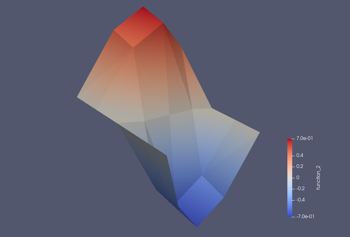
_images/level2.png — Fig. 1.1 Numerical solution on a \(4\times 4\) mesh.¶

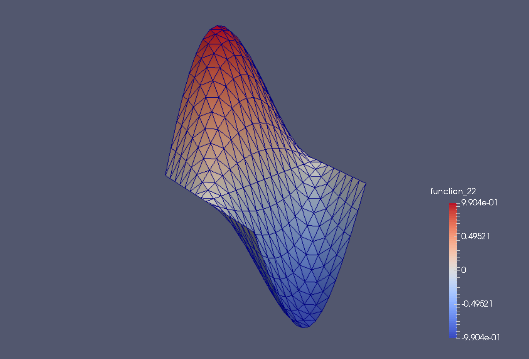
_images/level4.png — Fig. 1.2 Numerical solution on a \(16\times 16\) mesh.¶

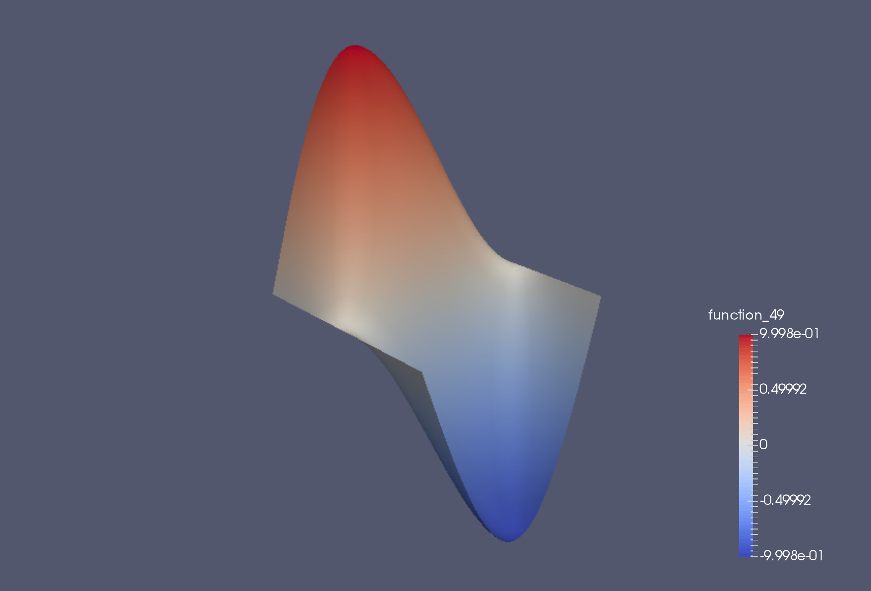
_images/level7.png — Fig. 1.3 Numerical solution on a \(128\times 128\) mesh.¶

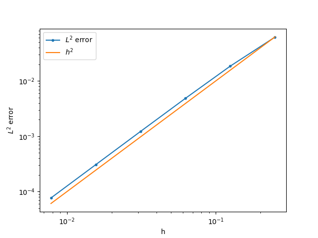
_images/poisson_error.png — Fig. 1.4 Plot showing error versus mesh resolution. We observe the error decreases proportionally to \(h^2\), where \(h\) is the maximum triangle edge size in the triangulation.¶

We see that for this example, the error is decreasing as we increase the number of triangles, for the meshes considered.

In general, our formulation raises a number of questions.

Is \(u_h\) unique?
What is the size of the error \(u-u_h\)?
Does this error go to zero as the mesh is refined?
For what types of functions \(f\) can these questions be answered?
What other kinds of finite element spaces are there?
How do we extend this approach to other PDEs?
How can we calculate \(u_h\) using a computer?

We shall aim to address these questions, at least partially, through the rest of this course. For now, we concentrate on the final question, in general terms.

In this course we shall mostly concentrate on finite element methods for elliptic PDEs, of which Poisson’s equation is an example, using continuous finite element spaces, of which \(P1\) is an example. The design, analysis and implementation of finite methods for PDEs is a huge field of current research, and includes parabolic and elliptic PDEs and other PDEs from elasticity, fluid dynamics, electromagnetism, mathematical biology, mathematical finance, astrophysics and cosmology, etc. This course is intended as a starting point to introduce the general concepts that can be applied in all of these areas.

Exercise 1.11

Derive a finite element approximation for the following problem.

Find \(u\) such that

\[-\nabla\cdot \left((2+\sin(2\pi x))\nabla u\right) = \exp(\cos(2\pi x)),\]

with boundary conditions \(u=0\) on the entire boundary.

Exercise 1.12

Derive a finite element approximation for the following problem.

Find \(u\) such that

\[-\nabla^2 u = \exp(xy),\]

in the \(1\times 1\) square region as above, with boundary conditions \(u=x(1-x)\) on the entire boundary.

Exercise 1.13

Derive a finite element approximation for the following problem.

Find \(u\) such that

\[-\nabla^2 u = \frac{1}{1 + x^2 + y^2},\]

in the \(1\times 1\) square region, with boundary conditions \(u+\frac{\partial u}{\partial n}=x(1-x)\) on the entire boundary.

1.7. Practical implementation¶

The finite element approximation above is only useful if we can actually compute it. To do this, we need to construct an efficient basis for \(P1\), which we call the nodal basis.

Definition 1.14 (P1 nodal basis)

Let \(\{z_i\}_{i=1}^{M}\) indicate the vertices in the triangulation \(\mathcal{T}\). For each vertex \(z_i\), we define a basis function \(\phi_i\in V_h\) by

\[\begin{split}\phi_i(z_j) = \delta_{ij} := \left\{ \begin{array}{cc} 1 & i=j, \\ 0 & i\ne j. \end{array} \right.\end{split}\]

We can define a similar basis for \(\mathring{V}_h\) by removing the basis functions \(\phi_i\) corresponding to vertices \(z_i\) on the Dirichlet boundaries \(x=0\) and \(x=1\); the dimension of the resulting basis is \(\bar{M}\).

If we expand \(u_h\) and \(v\) in the basis for \(\mathring{V}_h\),

\[u_h(x) = \sum_{i=1}^{\bar{M}}u_i\phi_i(x), \quad v(x) = \sum_{i=1}^{\bar{M}}v_i\phi_i(x),\]

into Equation (1.3), then we obtain

\[\sum_{i=1}^{\bar{M}}v_i\left(\sum_{j=1}^{\bar{M}}\int_\Omega \nabla \phi_i\cdot \nabla \phi_j \,dx u_j - \int_\Omega \phi_if\,dx\right) = 0.\]

Since this equation must hold for all \(v\in \mathring{V}_h\), then it must hold for all basis coefficients \(v_i\), and we obtain the matrix-vector system

\[K\mathrm{u} = \mathrm{f},\]

where

\[ \begin{align}\begin{aligned}K_{ij} = \int_\Omega \nabla\phi_i\cdot\nabla\phi_j\, d x,\\\mathrm{u} = \left(u_1,u_2,\ldots,u_{\bar{M}}\right)^T,\\\mathrm{f} = \left(f_1,f_2,\ldots,f_{\bar{M}}\right)^T, \quad f_i = \int_\Omega \phi_i f\, d x.\end{aligned}\end{align} \]

Once we have solved for \(\mathrm{u}\), we can use these basis coefficients to reconstruct the solution \(u_h\). The system is square, but we do not currently know that \(K\) is invertible. This is equivalent to the finite element approximation having a unique solution \(u_h\), which we shall establish in later sections. This motivates why we care that \(u_h\) exists and is unique.

Putting solvability aside for the moment, the goal of the implementation sections of this course is to explain how to efficiently form \(K\) and \(\mathrm{f}\), and solve this system. For now we note a few following aspects that suggest that this might be possible. First, the matrix \(K\) and vector \(\mathrm{f}\) can be written as sums over elements,

\[ \begin{align}\begin{aligned}K_{ij} = \sum_{K\in\mathcal{T}}\int_K \nabla \phi_i\cdot\nabla \phi_j \, d x,\\\mathrm{where}\,f_i = \sum_{K\in\mathcal{T}}\int_K \phi_i f \, d x.\end{aligned}\end{align} \]

For each entry in the sum for \(K_{ij}\), the integrand is composed entirely of polynomials (actually constants in this particular case, but we shall shortly consider finite element spaces using polynomials of higher degree). This motivates our starting point in exposing the computer implementation, namely the integration of polynomials over triangles using quadrature rules. This will also motivate an efficient way to construct derivatives of polynomials evaluated at quadrature points. Further, we shall shortly develop an interpolation operator \(\mathcal{I}\) such that \(\mathcal{I}_f\in V_h\). If we replace \(f\) by \(\mathcal{I}_f\) in the approximations above, then the evaluation of \(f_i\) can also be performed via quadrature rules.

Even further, the matrix \(K\) is very sparse, since in most triangles, both \(\phi_i\) and \(\phi_j\) are zero. Any efficient implementation must make use of this and avoid computing integrals that return zero. This motivates the concept of global assembly, the process of looping over elements, computing only the contributions to \(K\) that are non-zero from that element. Finally, the sparsity of \(K\) means that the system should be solved using numerical linear algebra algorithms that can exploit this sparsity.

Having set out the main challenges of the computational implementation, we now move on to define and discuss a broader range of possible finite element spaces.