9. Mixed problems

Note

This section is the mastery exercise for this module. This exercise is explicitly intended to test whether you can bring together what has been learned in the rest of the module in order to go beyond what has been covered in lectures and labs.

This exercise is not a part of the third year version of this module.

As an example of a mixed problem, let’s take the Stokes problem presented in Section 6 of the analysis part of the course. The weak form of the Stokes problem presented in Definition 6.1 is find \((u,p)\in V\times Q\) such that:

(9.1)\[ \begin{align}\begin{aligned}a(u,v) + b(v, p) & = \int_\Omega f\cdot v\,\mathrm{d}\, x,\\b(u,q) & = 0, \quad \forall (v,q) \in V\times Q,\end{aligned}\end{align} \]

where

(9.2)\[ \begin{align}\begin{aligned}a(u,v) & = \mu\int_\Omega \epsilon(u):\epsilon(v)\,\mathrm{d}\, x,\\b(v,q) & = \int_\Omega q \nabla\cdot v\,\mathrm{d}\, x,\\V & =(\mathring{H}^1(\Omega))^d,\\Q & =\mathring{L}^2(\Omega),\end{aligned}\end{align} \]

and where \((\mathring{H}^1(\Omega))^d\) is the subspace of \(H^1(\Omega)^d\) for which all components vanish on the boundary, and \(\mathring{L}^2(\Omega)\) is the subspace of \(L^2(\Omega)\) for which the integral of the function over the domain vanishes. This last constraint was introduced to remove the null space of constant pressure functions from the system. This constraint introduces a little complexity into the implementation. So instead, we will redefine \(\mathring{L}^2(\Omega)\) to be the subspace of \(L^2(\Omega)\) constrained to take the value 0 at some arbitrary but specified point. For example, one might choose to require the pressure at the origin to vanish. This is also an effective way to remove the nullspace, but it is simpler to implement. We will implement the two-dimensional case (\(d=2\)) and, for simplicity, we will assume \(\mu=1\).

The colon (\(:\)) indicates an inner product so:

(9.3)\[\epsilon(u):\epsilon(v) = \sum_{\alpha\beta} \epsilon(u)_{\alpha\beta}\epsilon(v)_{\alpha\beta}\]

In choosing a finite element subspace of \(V \times Q\) we will similarly choose a simpler to implement, yet still stable, space than was chosen in Analysis Section 6. The space we will use is the lowest order Taylor-Hood space [TH73]. This has:

(9.4)\[ \begin{align}\begin{aligned}V^h & = P2(\Omega)^2\\Q^h & = P1(\Omega)\end{aligned}\end{align} \]

i.e. quadratic velocity and linear pressure on each cell. We note that \(Q^h\in H^1(\Omega)\) but since \(H^1(\Omega) \subset L^2(\Omega)\), this is not itself a problem. We will impose further constraints on the spaces in the form of Dirichlet boundary conditions to ensure that the solutions found are in fact in \(V \times Q\).

In addition to the finite element functionality we have already implemented, there are two further challenges we need to address. First, the implementation of the vector-valued space \(P2(\Omega)^2`m and second, the implementation of functions and matrices defined over the mixed space `V^h \times Q^h\).

9.1. Vector-valued finite elements

Consider the local representation of \(P2(\Omega)^2\) on one element. The scalar \(P2\) element on one triangle has 6 nodes, one at each vertex and one at each edge. If we write \(\{\Phi_i\}_{i=0}^{5}\) for the scalar basis, then a basis \(\{\mathbf{\Phi}_i\}_{i=0}^{11}\) for the vector-valued space is given by:

(9.5)\[\mathbf{\Phi}_i(X) = \Phi_{i\,//\,2}(X)\,\mathbf{e}_{i\,\%\,2}\]

where \(//\) is the integer division operator, \(\%\) is the modulus operator, and \({\mathbf{e}_0, \mathbf{e}_1}\) is the standard basis for \(\mathbb{R}^2\). That is to say, we interleave \(x\) and \(y\) component basis functions.

Fig. 9.1 The local numbering of vector degrees of freedom.

We can practically implement vector function spaces by implementing a new class fe_utils.finite_elements.VectorFiniteElement. The constructor (__init__()) of this new class should take a FiniteElement and construct the corresponding vector element. For current purposes we can assume that the vector element will always have a vector dimension equal to the element geometric and topological dimension (i.e. 2 if the element is defined on a triangle). We’ll refer to this dimension as \(d\).

9.1.1. Implementing VectorFiniteElement

VectorFiniteElement needs to implement as far as possible the same interface as FiniteElement. Let’s think about how to do that.

cell, degree

Same as for the input FiniteElement.

entity_nodes

There will be twice as many nodes, and the node ordering is such that each node is replaced by a \(d\)-tuple. For example the scalar triangle P1 entity-node list is:

{
    0 : {0 : [0], 1 : [1], 2 : [2]},
    1 : {0 : [], 1 : [], 2 : []},
    2 : {0 : []}
}

The vector version is achieved by looping over the scalar version and returning a mapping with the pair \(2n, 2(n+1)\) in place of node \(n\):

{
    0 : {0 : [0, 1], 1 : [2, 3], 2 : [4, 5]},
    1 : {0 : [], 1 : [], 2 : []},
    2 : {0 : []}
}

nodes_per_entity:

Each entry will be \(d\) times that on the input FiniteElement.

9.1.2. Tabulation

In order to tabulate the element, we can use (9.5). We first call the tabulate method from the input FiniteElement, and we use this and (9.5) to produce the array to return. Notice that the array will both have a basis functions dimension which is \(d\) times longer than the input element, and will also have an extra dimension to account for the multiplication by \(\mathbf{e}_{i\,\%\,d}\). This means that the tabulation array with grad=False will now be rank 3, and that with grad=True will be rank 4. Make sure you keep track of which rank is which! The VectorFiniteElement will need to keep a reference to the input FiniteElement in order to facilitate tabulation.

9.1.3. Nodes

Even though we didn’t need the nodes of the VectorFiniteElement to construct its basis, we will need them to implement interpolation. In Definition 2.44 we learned that the nodes of a finite element are related to the corresponding nodal basis by:

(9.6)\[\mathbf{\Phi}^*_i(\mathbf{\Phi}_j) = \delta_{ij}\]

From (9.5) and assuming, as we have throughout the course, that the scalar finite element has point evaluation nodes given by:

(9.7)\[\Phi_i(v) = v(X_i),\]

it follows that:

(9.8)\[ \begin{align}\begin{aligned}\mathbf{\Phi}^*_i(v) & = \Phi^*_{i\,//\,d}(\mathbf{e}_{i\,\%\,d}\cdot v)\\& = \mathbf{e}_{i\,\%\,d}\cdot v(X_{i\,//\,d})\end{aligned}\end{align} \]

Hint

To see that this is the correct nodal basis, choose \(v=\mathbf{\Phi}_j\) in (9.8) and substitute (9.5) for \(\mathbf{\Phi}_j\).

This means that the correct VectorFiniteElement.nodes attribute is the list of nodal points from the input FiniteElement but with each point repeated \(d\) times. It will also be necessary to add another attribute, perhaps node_weights which is a rank 2 array whose \(i\)-th row is the correct canonical basis vector to contract with the function value at the \(i\)-th node (\(\mathbf{e}_{i\,\%\,d}\)).

9.2. Vector-valued function spaces

Assuming we correctly implement VectorFiniteElement, FunctionSpace should work out of the box. In particular, the global numbering algorithm only depends on having a correct local numbering so this should work unaltered.

9.3. Functions in vector-valued spaces

The general form of a function in a vector-valued function space is:

(9.9)\[f = f_i \mathbf{\Phi}_i(X).\]

That is to say, the basis functions are vector valued and their coefficients are still scalar. This means that if the VectorFiniteElement had a correct entity-node list then the core functionality of the existing Function will automatically be correct. In particular, the array of values will have the correct extent. However, interpolation and plotting of vector valued fields will require some adjustment.

9.3.1. Interpolating into vector-valued spaces

Since the form of the nodes of a VectorFiniteElement is different from that of a scalar element, there will be some changes required in the interpolate() method. Specifically:

self.values[fs.cell_nodes[c, :]] = [fn(x) for x in node_coords]

This line will need to take into account the dot product with the canonical basis from (9.8), which you have implemented as VectorFiniteElement.node_weights. This change will need to be made conditional on the class of finite element passed in, so that the code doesn’t break in the scalar element case.

9.3.2. Plotting functions in vector-valued spaces

The coloured surface plots that we’ve used thus far for two-dimensional scalar functions don’t extend easily to vector quantities. Instead, a frequently used visualisation technique is the quiver plot. This draws a set of arrows representing the function value at a set of points. For our purposes, the nodes of the function space in question are a good choice of evaluation points. Listing 9.1 provides the code you will need. Notice that at line 3 we interpolated the function \(f(x)=x\) into the function space in order to obtain a list of the global coordinates of the node locations. At lines 6 and 7 we use what we know about the node ordering to recover vector values from the list of basis function coefficients.

Listing 9.1 Code implementing quiver plots to visualise functions in vector function spaces. This code should be added to plot() immediately after the definition of fs.

if isinstance(fs.element, VectorFiniteElement):
    coords = Function(fs)
    coords.interpolate(lambda x: x)
    fig = plt.figure()
    ax = fig.add_subplot()
    x = coords.values.reshape(-1, 2)
    v = self.values.reshape(-1, 2)
    plt.quiver(x[:, 0], x[:, 1], v[:, 0], v[:, 1])
    plt.show()
    return

Once this code has been inserted, then running the code in Listing 9.2 will result in a plot rather like Fig. 9.2.

Listing 9.2 Creation of a vector function space, interpolation of a given function into it, and subsequent plot creation.

from fe_utils import *
from math import cos, sin, pi

se = LagrangeElement(ReferenceTriangle, 2)
ve = VectorFiniteElement(se)
m = UnitSquareMesh(10,10)
fs = FunctionSpace(m, ve)
f = Function(fs)
f.interpolate(lambda x: (2*pi*(1 - cos(2*pi*x[0]))*sin(2*pi*x[1]),
                         -2*pi*(1 - cos(2*pi*x[1]))*sin(2*pi*x[0])))
f.plot()

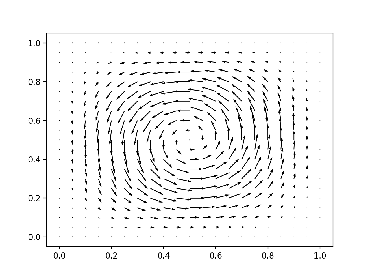
Fig. 9.2 The quiver plot resulting from Listing 9.2.

9.3.3. Solving vector-valued systems

Solving a finite element problem in a vector-valued space is essentially similar to the scalar problems you have already solved. It does, nonetheless, provide a useful check on the correctness of your code before adding in the additional complications of mixed systems. As a very simple example, consider computing vector-valued field which is the gradient of a known function. For some suitable finite element space \(V\subset H^1(\Omega)^2\) and \(f:\Omega\rightarrow \mathbb{R}\), find \(u\in V\) such that:

(9.10)\[\int_\Omega u\cdot v\,\mathrm{d}x = \int_\Omega \nabla f\cdot v\,\mathrm{d}x\quad \forall v\in V.\]

If \(f\) is chosen such that \(\nabla f\in V\) then this projection is exact up to roundoff, and the following calculation should result in a good approximation to zero:

(9.11)\[e = \int_\Omega (u -\nabla f)\cdot(u -\nabla f)\,\mathrm{d}x\]

Note

The computations in this subsection are not required to complete the mastery exercise. They are, nonetheless, strongly recommended as a mechanism for checking your implementation thus far.

9.4. Mixed function spaces

The Stokes equations are defined over the mixed function space \(W = V \times Q\). Here “mixed” simply means that there are two solution variables, and therefore two solution spaces. Functions in \(W\) are pairs \((u, p)\) where \(u\in V\) and \(p\in Q\). If \(\{\phi_i\}_{i=0}^{m-1}\) is a basis for \(V\) and \(\{\psi_j\}_{j=0}^{n-1}\) then a basis for \(W\) is given by:

(9.12)\[\{\omega_i\}_{i=0}^{m+n-1}=\{(\phi_i, 0)\}_{i=0}^{m-1} \cup \{(0, \psi_{j-n})\}_{j=m}^{m+n-1}.\]

This in turn enables us to write \(w\in W\) in the form \(w=w_i\omega_i\) as we would expect for a function in a finite element space. The Cartesian product structure of the mixed space \(W\) means that the first \(m\) coefficients are simply the coefficients of the \(V\) basis functions, and the latter \(n\) coefficients correspond to the \(Q\) basis functions. This means that our full mixed finite element system is simply a linear system of block matrices and block vectors. If we disregard boundary conditions, including the pressure constraint, this system has the following form:

(9.13)\[\begin{split}\begin{bmatrix} A & B^\mathrm{T} \\ B & 0 \end{bmatrix} \begin{bmatrix} U \\ P \end{bmatrix} = \begin{bmatrix} F \\ 0 \end{bmatrix}\end{split}\]

where:

(9.14)\[ \begin{align}\begin{aligned}A_{ij} = a(\phi_j, \phi_i),\\B_{ij} = b(\phi_j, \psi_i),\\F_i = \int_\Omega f\cdot v\, d\, x,\\U_i = u_i = w_i,\\P_i = p_i = w_{i+m}.\end{aligned}\end{align} \]

This means that the assembly of the mixed problem comes down to the assembly of several finite operators of the form that we have already encountered. These then need to be assembled into the full block matrix and right hand side vector, before the system is solved and the resulting solution vector pulled appart and interpreted as the coefficients of \(u\) and \(p\). Observe in (9.14) that the order of the indices \(i\) and \(j\) is reversed on the right hand side of the equations. This reflects the differing conventions for matrix indices and bilinear form arguments, and is a source of unending confusion in this field.

9.4.1. Assembling block systems

The procedure for assembling the individual blocks of the block matrix and the block vectors is the one you are familiar with, but we will need to do something new to assemble the block structures. What is required differs slightly between the matrix and the vectors.

In the case of the vectors, then it is sufficient to know that a slice into a numpy.ndarray returns a view on the same memory as the full vector. This is most easily understood through an example:

In [1]: import numpy as np

In [2]: a = np.zeros(10)

In [3]: b = a[:5]

In [4]: b[2] = 1

In [5]: a
Out[5]: array([0., 0., 1., 0., 0., 0., 0., 0., 0., 0.])

This means that one can first create a full vector of length \(n+m\) and then slice it to create subvectors that can be used for assembly.

Conversely, scipy.sparse provides the bmat() function which will stitch together a larger sparse matrix from blocks. In order to have the full indexing options you are likely to want for imposing the boundary conditions, you will probably want to specify that the resulting matrix is in "lil" format.

9.4.2. Boundary conditions

The imposition of the constraint in \((\mathring{H}^1(\Omega))^2\) that solutions vanish on the boundary is a Dirichlet condition of the type that you have encountered before. Observe that the condition changes the test space, which affects whole rows of the block system, so you will want to impose the boundary condition after assembling the block matrix. You will also need to ensure that the constraint is applied to both the \(x\) and \(y\) components of the space.

The imposition of the constraint in \(\mathring{L}^2(\Omega)\) that the solution is zero at some prescribed point can be achieved by selecting an arbitrary basis function and applying a zero Dirichlet condition for that degree of freedom. In this regard we can observe that there is nothing about the implementation of Dirichlet conditions that constrains them to lie on the boundary. Rather, they should be understood as specifying a subspace on which the solution is prescribed rather than solved for. In this particular case, that subspace is one-dimensional.

9.4.3. Solving the matrix system

The block matrix system that you eventually produce will be larger than many of those we have previously encountered, and will have non-zero entries further from the diagonal. This can cause the matrix solver to become expensive in both time and memory. Fortunately, scipy.sparse.linalg now incorporates an interface to SuperLU, which is a high-performance direct sparse solver. The recommended solution strategy is therefore:

1. Convert your block matrix to scipy.sparse.csc_matrix, which is the format that SuperLU requires.

2. Factorise the matrix using scipy.sparse.linalg.splu().

3. Use the resulting SuperLU object to finally solve the system.

9.4.4. Computing the error

We will wish to compute the convergence of our solution in the \(L^2\) norm. For \(w\in W\), this is given by:

(9.15)\[\|w\|_{L^2} = \sqrt{\int_\Omega w\cdot w\,\mathrm{dx}}\]

When we expand this in terms of the basis of \(W\), it will be useful to note that basis functions from the different component spaces are orthogonal. That is to say:

(9.16)\[(\phi, 0) \cdot (0, \psi) = 0 \quad \forall \phi\in V,\, \psi \in Q.\]

The direct result of this is that if \(w = (u, p)\) then:

(9.17)\[\|w\|_{L^2}^2 = \|u\|_{L^2}^2 + \|p\|_{L^2}^2.\]

9.5. Manufacturing a solution to the Stokes equations

As previously, we will wish to check our code using the method of manufactured solutions. The Stokes equations represent a form of incompressible fluid mechanics, so it is usually preferable to select a target solution for which \(\nabla\cdot u = 0\). The straightforward way to do this is to choose a scalar field \(\gamma: \Omega\rightarrow \mathbb{R}\) to use as a streamfunction. We can then define \(u = \nabla^{\perp}\gamma\) and rely on the vector calculus identity \(\nabla\cdot\nabla^{\perp} \gamma = 0\) to guarantee that the velocity field is divergence-free. We also need to ensure that \(u\) satisfies the boundary conditions, which amounts to choosing \(\gamma\) such that its gradient vanishes on the domain boundary. The following function is a suitable choice on a unit square domain:

(9.18)\[\gamma(x,y) = \big(1-\cos(2\pi x)\big)\big(1-\cos(2\pi y)\big)\]

9.6. Implementing the Stokes problem

Exercise 9.1

The goal of this exercise is to implement a solver for the Stokes equations, on a unit square. Implement solve_mastery() so that it solves (9.1) using the forcing function derived from (9.18).

Your full solution should:

1. Implement VectorFiniteElement.

2. Make the consequential changes to Function to enable values to be interpolated into vector-valued functions, and to create quiver plots.

3. Assemble and solve the required mixed system.

4. Compute the \(L^2\) error of the mixed solution from the analytic solution.

A convergence test for your code is provided in test/test_13_mastery_convergence.py. In order to be compatible with this code, your implementation of solve_mastery() should return its results as a tuple of the form (u, p), error. This is a slight change from the comment in the code which takes into account that the problem is mixed. The obvious consequential change will be needed at the end of fe_utils.solvers.mastery.